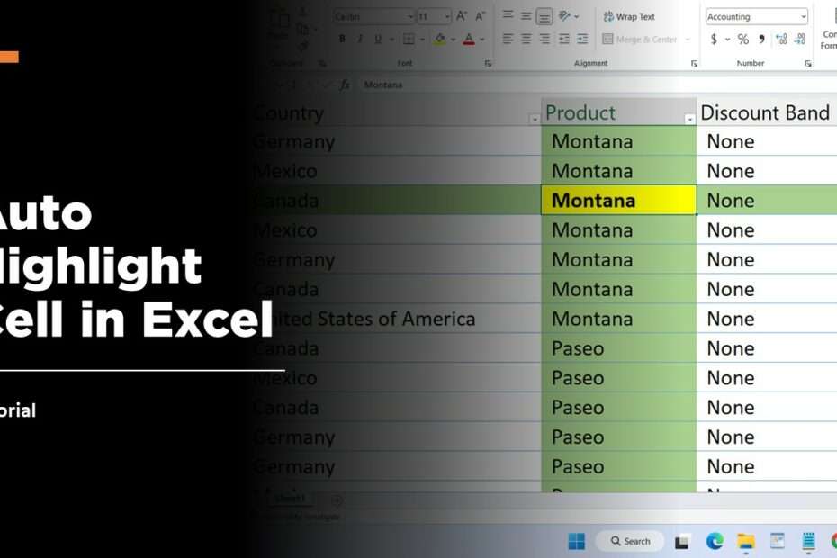
When you have a lot of data in Microsoft Excel, a feature that may be very useful to you is auto-highlight on the active cell we selected. This will make it easier for us to identify data so as to minimize errors in seeing one data with another. The auto-highlight feature on the active cell is not in Microsoft Excel by default, but we can create it with a simple formula.
This auto-highlight feature will highlight cells horizontally, while the cursor where you click cells can style them to your liking. For example, you can use a certain background color, a certain font style, and so on. To create an automatic highlight feature on the active cell in Microsoft Excel you can follow the following guide.
How to Create Auto Highlight on The Active Cell in Microsoft Excel
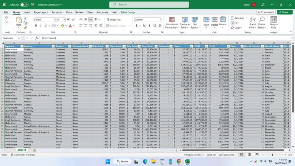
- Open a sheet in Microsoft Excel, create some data as an example and select/block the data.
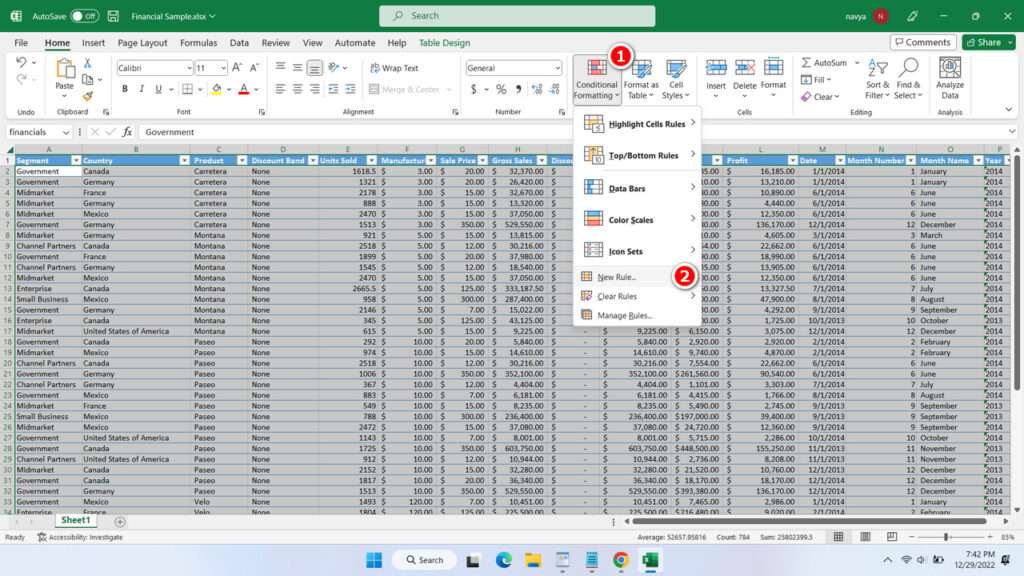
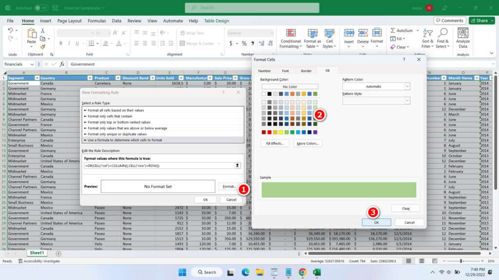
- Click “Conditional Formatting” > “New Rule“. Select the option “Use a fromula to determine which cells to format“.
- Enter the following formula in the formula field (select the one that works, because writing the formula depends on the installation of your Windows system, some work with semicolon “;” and some work with comma “,“).
Choose one
=OR(CELL("col")=COLUMN(),CELL("row")=ROW())or
=OR(CELL("col")=COLUMN();CELL("row")=ROW())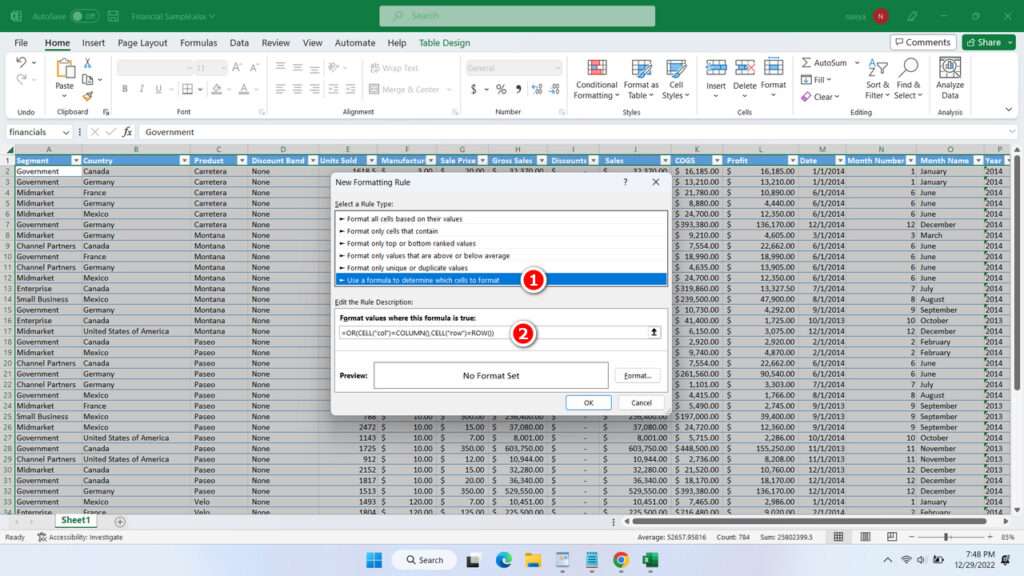
- Click the “Format” button, click the “Fill” tab, select the color you like then click “OK“.
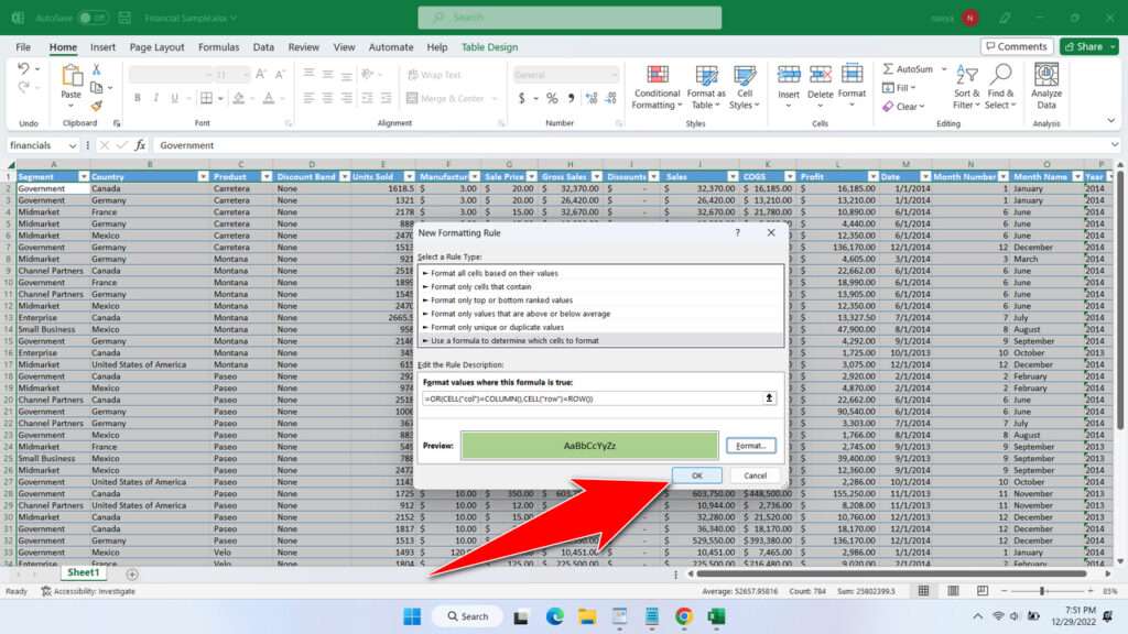
- Click “OK” to save the formula and highlight color.
- Repeat the steps to enter one of the following formulas as the previous step. But this formula begins with the condition “AND“. Select “Conditional Formatting” > “New Rule“, select the same option under “Use a fromula to determine which cells to format“. Select the color on the “Format” button > “Fill” with the color to be used in the active cell, here I choose yellow. If you have done please click “OK“.
Choose one
=AND(CELL("col")=COLUMN(),CELL("row")=ROW())or
=AND(CELL("col")=COLUMN();CELL("row")=ROW())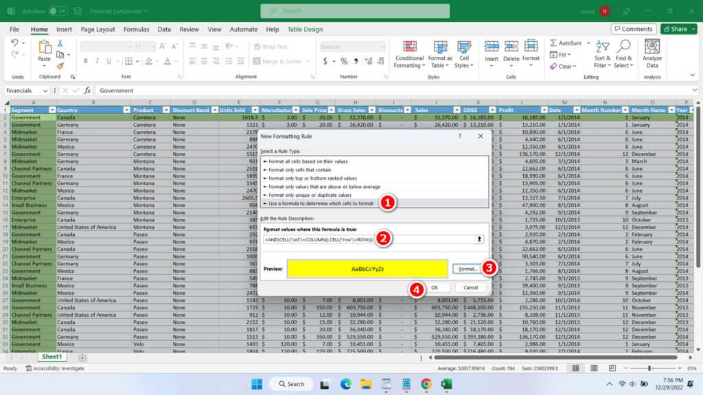
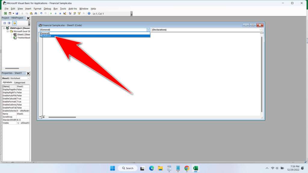
- In your sheet tab click “View Code“. Select the “Worksheet” option. Enter the following code among the Private Subs. After that you can close the VBA Code.
Target.Calculate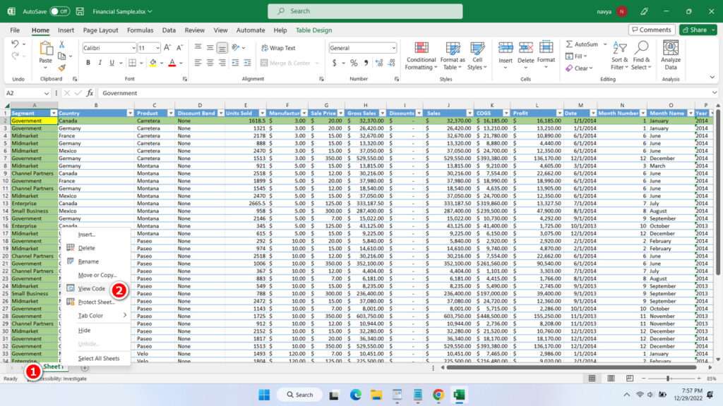
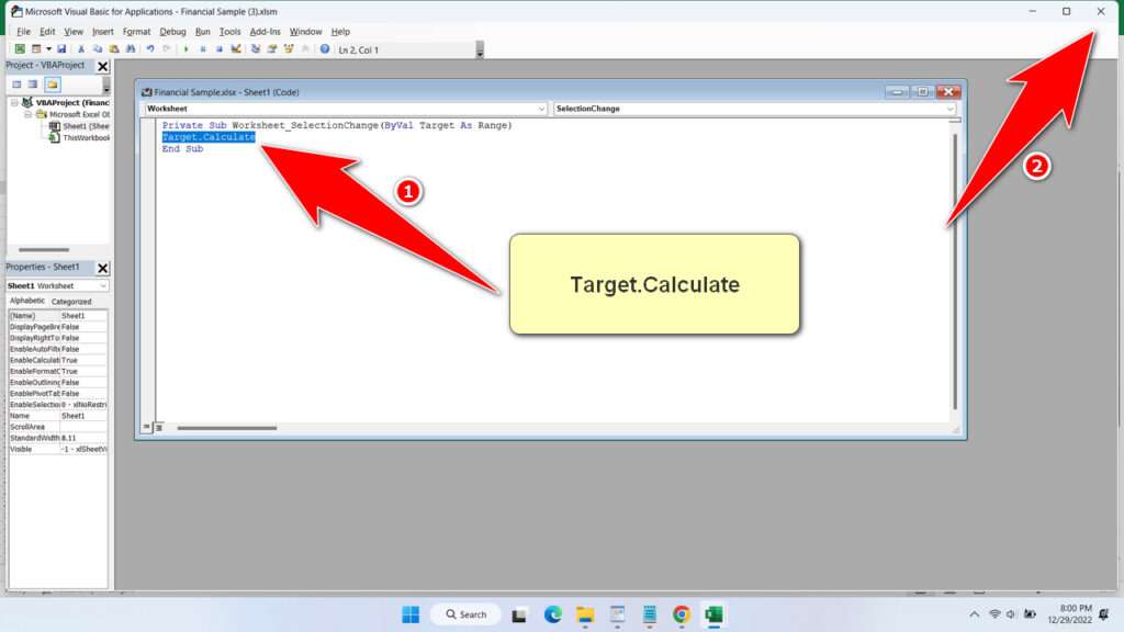
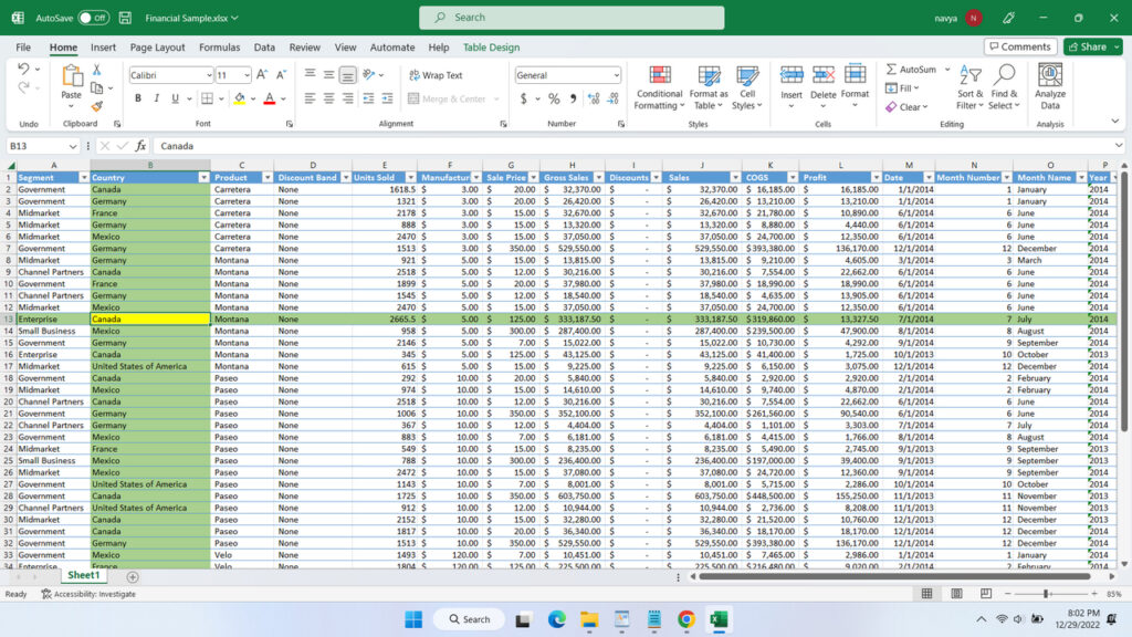
- You have successfully created an automatic highlight in Microsoft Excel.
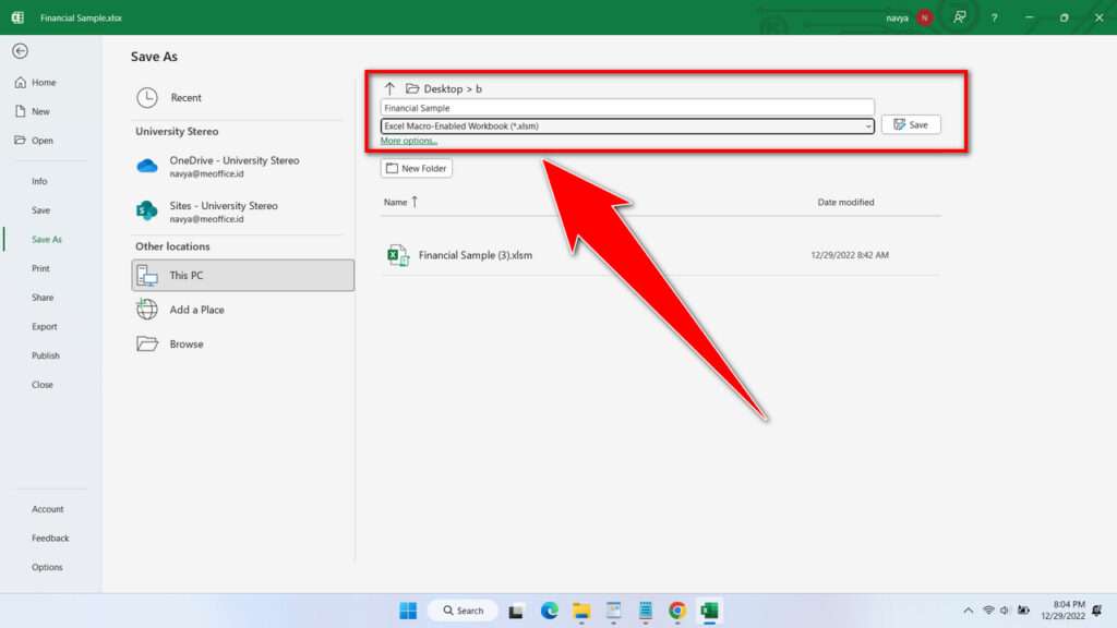
- To keep the VBA Code stored properly, save the file as a macro by clicking “File” > “Save As” > select “Excel Macro-Enabled Workbook (*.xlsm)“.
- You may also need to allow macros to be automatically loaded in excel settings so that the file can be opened normally at a later time, this menu is located in “Trust Center Settings” in Microsoft Excel Options.
That’s a guide on how to create an automatic highlight on the active cell in Microsoft Excel using formulas and also VBA codes. You can also see the guide in the following video.

